Read Data
data = read_csv('https://raw.githubusercontent.com/ariannalangwang/Analyze-HR-Data/master/HRDataProject/HRDataset_v13.csv') %>%
   clean_names()
data
## # A tibble: 310 × 35
## employee_name emp_id married_id marital_status_… gender_id emp_status_id
## <chr> <dbl> <dbl> <dbl> <dbl> <dbl>
## 1 Brown, Mia 1.10e9 1 1 0 1
## 2 LaRotonda, William 1.11e9 0 2 1 1
## 3 Steans, Tyrone 1.30e9 0 0 1 1
## 4 Howard, Estelle 1.21e9 1 1 0 1
## 5 Singh, Nan 1.31e9 0 0 0 1
## 6 Smith, Leigh Ann 7.11e8 1 1 0 5
## 7 Bunbury, Jessica 1.50e9 1 1 0 5
## 8 Carter, Michelle 1.40e9 0 0 0 1
## 9 Dietrich, Jenna 1.41e9 0 0 0 1
## 10 Digitale, Alfred 1.31e9 1 1 1 1
## # … with 300 more rows, and 29 more variables: dept_id <dbl>,
## # perf_score_id <dbl>, from_diversity_job_fair_id <dbl>, pay_rate <dbl>,
## # termd <dbl>, position_id <dbl>, position <chr>, state <chr>, zip <chr>,
## # dob <chr>, sex <chr>, marital_desc <chr>, citizen_desc <chr>,
## # hispanic_latino <chr>, race_desc <chr>, dateof_hire <chr>,
## # dateof_termination <chr>, term_reason <chr>, employment_status <chr>,
## # department <chr>, manager_name <chr>, manager_id <dbl>, …Explore Data
skimr::skim(data) #summary| Name | data |
| Number of rows | 310 |
| Number of columns | 35 |
| _______________________ | |
| Column type frequency: | |
| character | 19 |
| numeric | 16 |
| ________________________ | |
| Group variables | None |
Variable type: character
| skim_variable | n_missing | complete_rate | min | max | empty | n_unique | whitespace |
|---|---|---|---|---|---|---|---|
| employee_name | 0 | 1.00 | 8 | 23 | 0 | 310 | 0 |
| position | 0 | 1.00 | 3 | 28 | 0 | 31 | 0 |
| state | 0 | 1.00 | 2 | 2 | 0 | 28 | 0 |
| zip | 0 | 1.00 | 5 | 5 | 0 | 158 | 0 |
| dob | 0 | 1.00 | 8 | 8 | 0 | 306 | 0 |
| sex | 0 | 1.00 | 1 | 1 | 0 | 2 | 0 |
| marital_desc | 0 | 1.00 | 6 | 9 | 0 | 5 | 0 |
| citizen_desc | 0 | 1.00 | 10 | 19 | 0 | 3 | 0 |
| hispanic_latino | 0 | 1.00 | 2 | 3 | 0 | 4 | 0 |
| race_desc | 0 | 1.00 | 5 | 32 | 0 | 6 | 0 |
| dateof_hire | 0 | 1.00 | 8 | 10 | 0 | 99 | 0 |
| dateof_termination | 207 | 0.33 | 8 | 8 | 0 | 93 | 0 |
| term_reason | 1 | 1.00 | 5 | 32 | 0 | 17 | 0 |
| employment_status | 0 | 1.00 | 6 | 22 | 0 | 5 | 0 |
| department | 0 | 1.00 | 5 | 20 | 0 | 6 | 0 |
| manager_name | 0 | 1.00 | 8 | 18 | 0 | 21 | 0 |
| recruitment_source | 0 | 1.00 | 5 | 38 | 0 | 23 | 0 |
| performance_score | 0 | 1.00 | 3 | 17 | 0 | 4 | 0 |
| last_performance_review_date | 103 | 0.67 | 8 | 9 | 0 | 42 | 0 |
Variable type: numeric
| skim_variable | n_missing | complete_rate | mean | sd | p0 | p25 | p50 | p75 | p100 | hist |
|---|---|---|---|---|---|---|---|---|---|---|
| emp_id | 0 | 1.00 | 1.199745e+09 | 1.8296e+08 | 602000312.00 | 1.101024e+09 | 1.203032e+09 | 1.378814e+09 | 1988299991 | ▁▇▇▁▁ |
| married_id | 0 | 1.00 | 4.000000e-01 | 4.9000e-01 | 0.00 | 0.000000e+00 | 0.000000e+00 | 1.000000e+00 | 1 | ▇▁▁▁▅ |
| marital_status_id | 0 | 1.00 | 8.100000e-01 | 9.4000e-01 | 0.00 | 0.000000e+00 | 1.000000e+00 | 1.000000e+00 | 4 | ▇▇▂▁▁ |
| gender_id | 0 | 1.00 | 4.300000e-01 | 5.0000e-01 | 0.00 | 0.000000e+00 | 0.000000e+00 | 1.000000e+00 | 1 | ▇▁▁▁▆ |
| emp_status_id | 0 | 1.00 | 2.400000e+00 | 1.8000e+00 | 1.00 | 1.000000e+00 | 1.000000e+00 | 5.000000e+00 | 5 | ▇▁▁▁▃ |
| dept_id | 0 | 1.00 | 4.610000e+00 | 1.0800e+00 | 1.00 | 5.000000e+00 | 5.000000e+00 | 5.000000e+00 | 6 | ▁▂▁▇▁ |
| perf_score_id | 0 | 1.00 | 2.980000e+00 | 5.8000e-01 | 1.00 | 3.000000e+00 | 3.000000e+00 | 3.000000e+00 | 4 | ▁▁▁▇▁ |
| from_diversity_job_fair_id | 0 | 1.00 | 9.000000e-02 | 2.9000e-01 | 0.00 | 0.000000e+00 | 0.000000e+00 | 0.000000e+00 | 1 | ▇▁▁▁▁ |
| pay_rate | 0 | 1.00 | 3.128000e+01 | 1.5380e+01 | 14.00 | 2.000000e+01 | 2.400000e+01 | 4.531000e+01 | 80 | ▇▂▂▂▁ |
| termd | 0 | 1.00 | 3.300000e-01 | 4.7000e-01 | 0.00 | 0.000000e+00 | 0.000000e+00 | 1.000000e+00 | 1 | ▇▁▁▁▃ |
| position_id | 0 | 1.00 | 1.684000e+01 | 6.2300e+00 | 1.00 | 1.800000e+01 | 1.900000e+01 | 2.000000e+01 | 30 | ▂▁▁▇▁ |
| manager_id | 8 | 0.97 | 1.458000e+01 | 8.0900e+00 | 1.00 | 1.000000e+01 | 1.500000e+01 | 1.900000e+01 | 39 | ▅▇▇▁▁ |
| engagement_survey | 0 | 1.00 | 3.330000e+00 | 1.2900e+00 | 1.03 | 2.080000e+00 | 3.470000e+00 | 4.520000e+00 | 5 | ▅▅▃▅▇ |
| emp_satisfaction | 0 | 1.00 | 3.890000e+00 | 9.1000e-01 | 1.00 | 3.000000e+00 | 4.000000e+00 | 5.000000e+00 | 5 | ▁▁▇▇▇ |
| special_projects_count | 0 | 1.00 | 1.210000e+00 | 2.3500e+00 | 0.00 | 0.000000e+00 | 0.000000e+00 | 0.000000e+00 | 8 | ▇▁▁▂▁ |
| days_late_last30 | 103 | 0.67 | 0.000000e+00 | 0.0000e+00 | 0.00 | 0.000000e+00 | 0.000000e+00 | 0.000000e+00 | 0 | ▁▁▇▁▁ |
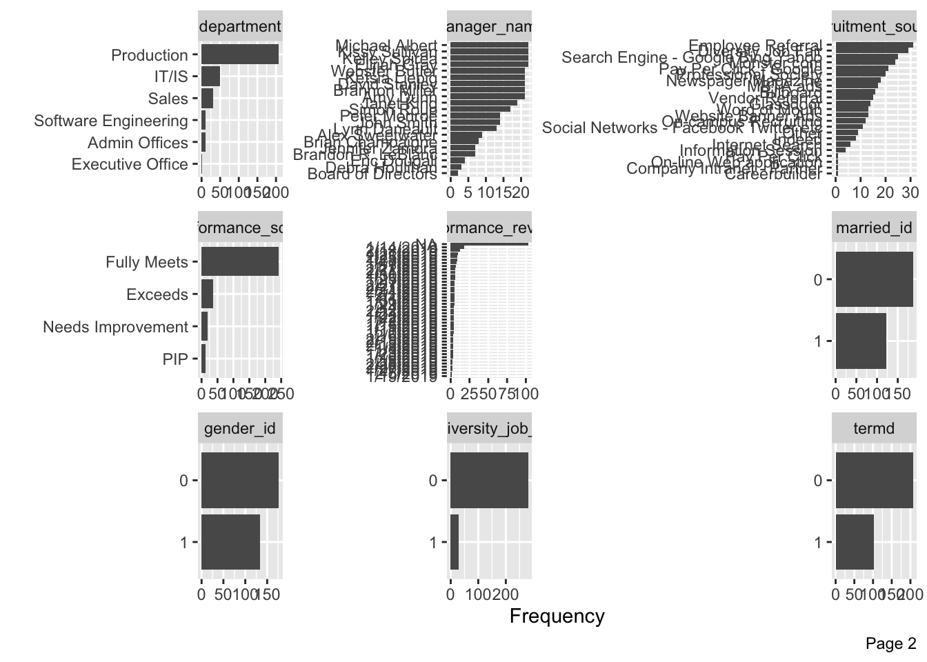
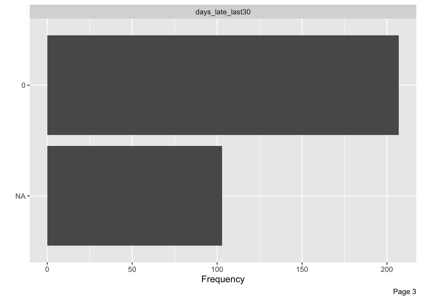
DataExplorer::plot_bar(data)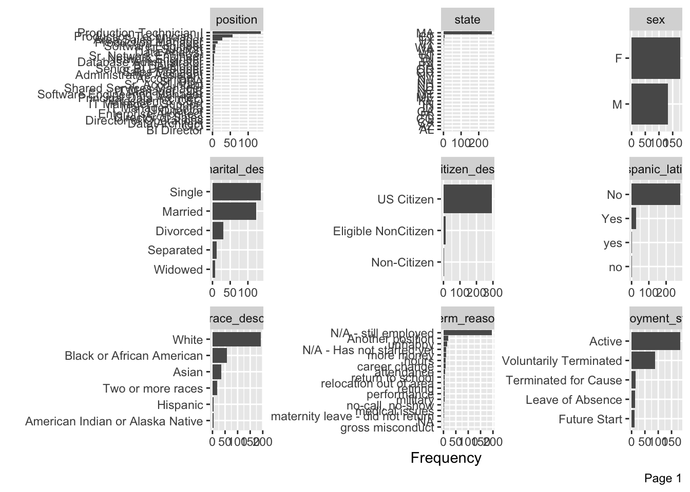
Pivot Table
rpivotTable::rpivotTable(data,
height = 1500)Check for duplicates
(nrow(get_dupes(data)) == 0) #duplicates?## [1] TRUECheck reduntant information
data %>% distinct(hispanic_latino)## # A tibble: 4 × 1
## hispanic_latino
## <chr>
## 1 No
## 2 Yes
## 3 yes
## 4 nodata <- data %>% mutate(
hispanic_latino = as_factor(hispanic_latino),
hispanic_latino = recode(data$hispanic_latino,
yes = 'Yes', no = 'No'))Missing data
#missing data?
data %>% miss_var_summary()
## # A tibble: 35 × 3
## variable n_miss pct_miss
## <chr> <int> <dbl>
## 1 dateof_termination 207 66.8
## 2 last_performance_review_date 103 33.2
## 3 days_late_last30 103 33.2
## 4 manager_id 8 2.58
## 5 term_reason 1 0.323
## 6 employee_name 0 0
## 7 emp_id 0 0
## 8 married_id 0 0
## 9 marital_status_id 0 0
## 10 gender_id 0 0
## # … with 25 more rowsdata %>% gg_miss_upset()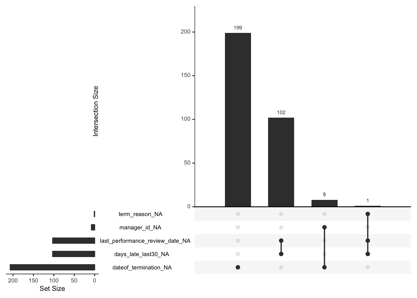
# plot missing data (using raw data)
DataExplorer::plot_missing(
  title   = "% of Missing Data",
  data    = data,
  ggtheme = tidyquant::theme_tq(),
missing_only = TRUE) 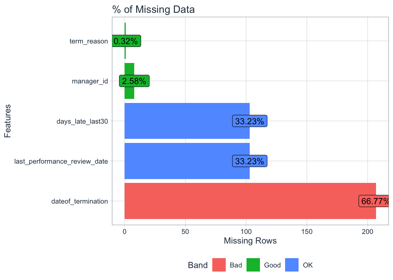
#Term Reason column
data %>% select(dateof_termination, term_reason) %>% count(term_reason,sort=T)
## # A tibble: 18 × 2
## term_reason n
## <chr> <int>
## 1 N/A - still employed 196
## 2 Another position 20
## 3 unhappy 14
## 4 more money 11
## 5 N/A - Has not started yet 11
## 6 career change 9
## 7 hours 9
## 8 attendance 7
## 9 relocation out of area 5
## 10 return to school 5
## 11 military 4
## 12 performance 4
## 13 retiring 4
## 14 maternity leave - did not return 3
## 15 medical issues 3
## 16 no-call, no-show 3
## 17 gross misconduct 1
## 18 <NA> 1#it seems there is a missing value here, we drop the row
data <- data %>% drop_na(term_reason)
#Manager ID
#Count how many employees has each manager
data %>% select(manager_name, manager_id) %>% count(manager_name,sort=T) ## # A tibble: 21 × 2
## manager_name n
## <chr> <int>
## 1 Elijiah Gray 22
## 2 Kelley Spirea 22
## 3 Kissy Sullivan 22
## 4 Michael Albert 22
## 5 Amy Dunn 21
## 6 Brannon Miller 21
## 7 David Stanley 21
## 8 Ketsia Liebig 21
## 9 Webster Butler 21
## 10 Janet King 19
## # … with 11 more rows#Which manager has not id values?
data %>% select(manager_name, manager_id) %>% filter(is.na(manager_id))## # A tibble: 8 × 2
## manager_name manager_id
## <chr> <dbl>
## 1 Webster Butler NA
## 2 Webster Butler NA
## 3 Webster Butler NA
## 4 Webster Butler NA
## 5 Webster Butler NA
## 6 Webster Butler NA
## 7 Webster Butler NA
## 8 Webster Butler NA# Webster Butler has not id, let'see if it applies for other rows.
data %>% select(manager_name, manager_id) %>% filter(manager_name == 'Webster Butler')## # A tibble: 21 × 2
## manager_name manager_id
## <chr> <dbl>
## 1 Webster Butler 39
## 2 Webster Butler NA
## 3 Webster Butler NA
## 4 Webster Butler 39
## 5 Webster Butler 39
## 6 Webster Butler 39
## 7 Webster Butler 39
## 8 Webster Butler 39
## 9 Webster Butler 39
## 10 Webster Butler 39
## # … with 11 more rows# As expected just few rows did not reported his id, so we impute with his reported id of 39
#fill with 39 where is.na == TRUE
data$manager_id[is.na(data$manager_id)] <- 39
data %>% select(dateof_termination,
last_performance_review_date,
days_late_last30)## # A tibble: 309 × 3
## dateof_termination last_performance_review_date days_late_last30
## <chr> <chr> <dbl>
## 1 <NA> 1/15/2019 0
## 2 <NA> 1/17/2019 0
## 3 <NA> 1/18/2019 0
## 4 <NA> 1/15/2019 0
## 5 09/25/13 <NA> NA
## 6 08/02/14 <NA> NA
## 7 <NA> 1/21/2019 0
## 8 <NA> 1/29/2019 0
## 9 <NA> 1/30/2019 0
## 10 <NA> 1/17/2019 0
## # … with 299 more rowsunique(data$days_late_last30)## [1] 0 NAdata %>% select(-days_late_last30)## # A tibble: 309 × 34
## employee_name emp_id married_id marital_status_… gender_id emp_status_id
## <chr> <dbl> <dbl> <dbl> <dbl> <dbl>
## 1 Brown, Mia 1.10e9 1 1 0 1
## 2 LaRotonda, William 1.11e9 0 2 1 1
## 3 Steans, Tyrone 1.30e9 0 0 1 1
## 4 Singh, Nan 1.31e9 0 0 0 1
## 5 Smith, Leigh Ann 7.11e8 1 1 0 5
## 6 Bunbury, Jessica 1.50e9 1 1 0 5
## 7 Carter, Michelle 1.40e9 0 0 0 1
## 8 Dietrich, Jenna 1.41e9 0 0 0 1
## 9 Digitale, Alfred 1.31e9 1 1 1 1
## 10 Friedman, Gerry 1.20e9 0 0 1 1
## # … with 299 more rows, and 28 more variables: dept_id <dbl>,
## # perf_score_id <dbl>, from_diversity_job_fair_id <dbl>, pay_rate <dbl>,
## # termd <dbl>, position_id <dbl>, position <chr>, state <chr>, zip <chr>,
## # dob <chr>, sex <chr>, marital_desc <chr>, citizen_desc <chr>,
## # hispanic_latino <chr>, race_desc <chr>, dateof_hire <chr>,
## # dateof_termination <chr>, term_reason <chr>, employment_status <chr>,
## # department <chr>, manager_name <chr>, manager_id <dbl>, …It seems that no employees came late in the last 30 days as the column days_late_last30 presents only 0 values and NA for the rows wherein the employee has already left the company. So I will drop the column.
unique(data[,c("dateof_termination","term_reason")])## # A tibble: 103 × 2
## dateof_termination term_reason
## <chr> <chr>
## 1 <NA> N/A - still employed
## 2 09/25/13 career change
## 3 08/02/14 Another position
## 4 09/05/15 attendance
## 5 10/31/14 relocation out of area
## 6 <NA> N/A - Has not started yet
## 7 09/12/15 performance
## 8 03/15/15 no-call, no-show
## 9 02/22/15 no-call, no-show
## 10 05/01/16 performance
## # … with 93 more rowsemployees <- data %>% filter(
is.na(dateof_termination)) %>%
select(-dateof_termination)
term_employees <- data %>% filter(
is.na(dateof_termination) == F)Data Visualization
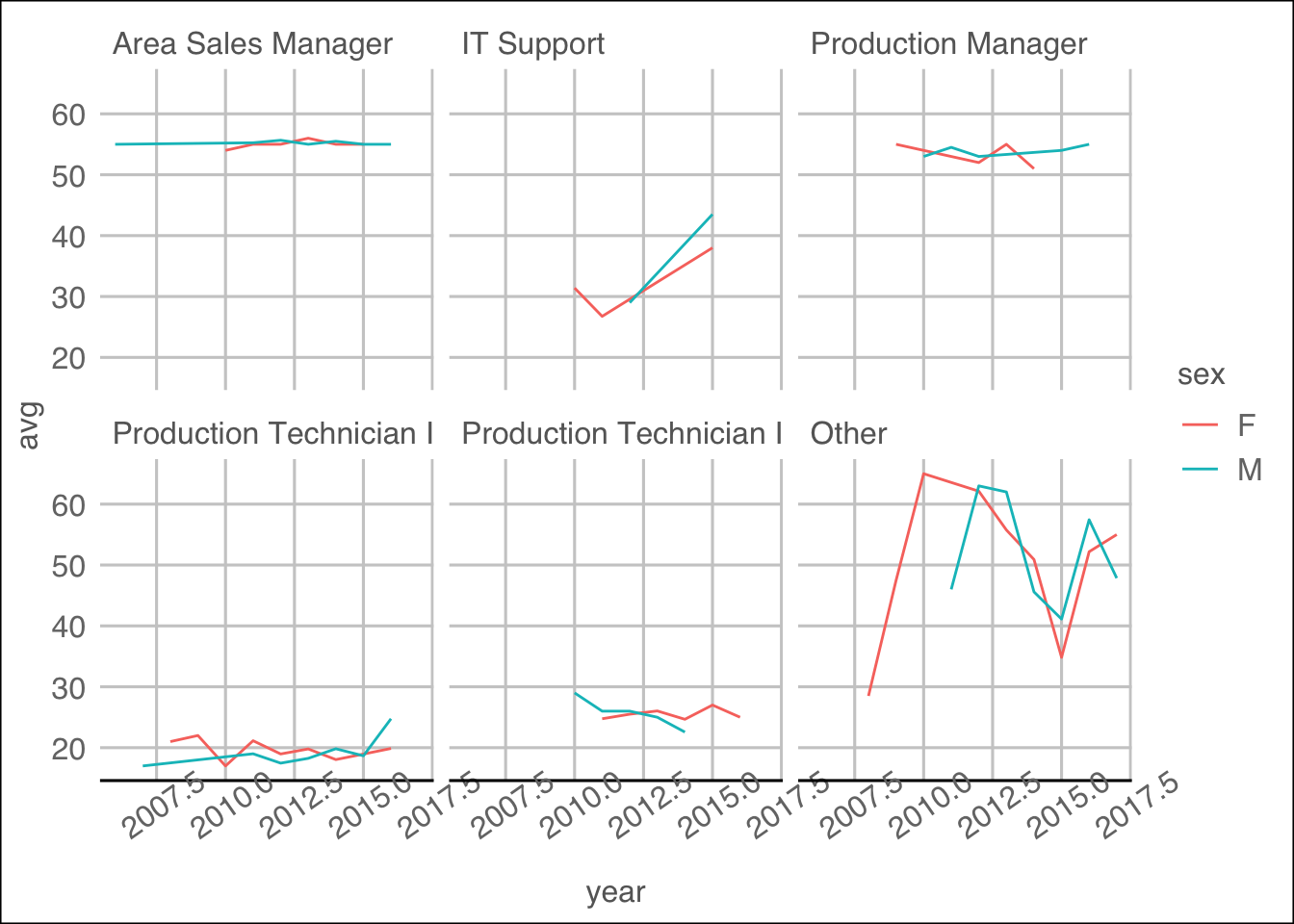
Gender Gap
employees %>% select(sex, pay_rate,
                    dateof_hire, position) %>% mutate(
        position = as.factor(position),
        position = fct_lump(position, 5),
        dateof_hire=anytime::anydate(dateof_hire),
        sex = as_factor(sex),
        year = year(dateof_hire)) %>%
group_by(year,sex, position) %>% summarise(
    avg = mean(pay_rate)) %>%
    ggplot(aes(x=year, y=avg, color =sex)) + geom_line() + facet_wrap(~position) + ggthemes::theme_gdocs() + theme(
        axis.text.x = element_text(angle = 35)
    )
Barplot
data %>%
  filter(term_reason=="N/A - still employed") %>%
  group_by(sex,position) %>%
  summarise(Total=n()) %>%
  hchart(type="column",
        hcaes(x=position,y=Total,group=sex)) %>%
hc_add_theme(hc_theme_economist())data %>% group_by(position) %>% summarise(pay_rate = round(mean(pay_rate),2)) %>%
hchart("column", hcaes(x = position, y = pay_rate)) %>%
hc_title(text = "Company Pay Rates") %>%
hc_subtitle(text = "Average pay rate by job position") %>%
hc_add_theme(hc_theme_economist())Boxplot
highchart() %>%
  hc_xAxis(type ="category")%>%
  hc_add_series_list(data_to_boxplot(data,
                                pay_rate, race_desc,
                                group_var = sex,
                                add_outliers = F)) %>%
  hc_legend(enabled= F) %>%
hc_add_theme(hc_theme_economist())Pie Charts
race_pie <- data %>% count(race_desc) %>%
    hchart('pie', hcaes(race_desc,n)) %>% hc_add_theme(hc_theme_economist())

gender_pie <- data %>% count(sex) %>%
    hchart('pie', hcaes(sex,n)) %>%
    hc_add_theme(hc_theme_economist())

department_pie <- data %>% count(department) %>%
    hchart('pie', hcaes(department, n)) %>%
    hc_add_theme(hc_theme_economist())

managers_pie <- data %>% count(manager_name) %>%
    hchart('pie', hcaes(manager_name, n)) %>%
    hc_add_theme(hc_theme_economist())

hw_grid(race_pie, gender_pie,
                department_pie, managers_pie,
ncol = 2, rowheight = 350)Waffle Plot
pacman::p_load(waffle)

View(employees %>% select(marital_desc,performance_score) %>%
            group_by(marital_desc,performance_score) %>%
    summarise(n= n()) %>% mutate(freq = round(n/sum(n),2)))

waffle(c('Exceeds = 15%' = 15,
                 'Fully Meets = 78%' =78,
                 'Needs Improvement = 4%' = 4,
                 'PIP = 3%' = 3),
             rows = 8, size = 0.2,
             title = 'Performance Score For Single Employees') +
    theme(title = element_text(
        family = 'Arial',
        size = 1, face = 'bold'
    ))
Ridgeline Plots
library(ggridges)
ggplot(data, aes(
    y=as_factor(race_desc),
    x=pay_rate,
    fill=sex
)) + geom_density_ridges(alpha=0.7) + theme_minimal()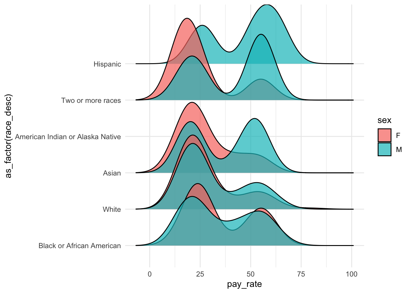
Treemap
data$manager_name <- as_factor(data$manager_name)

data %>% mutate(
    manager_name = fct_lump(manager_name,15)) %>%
    group_by(manager_name) %>% count() %>%
treemap::treemap(
    index = 'manager_name',
    vSize = 'n',
    title = "Treemap: Managers names by number of employees")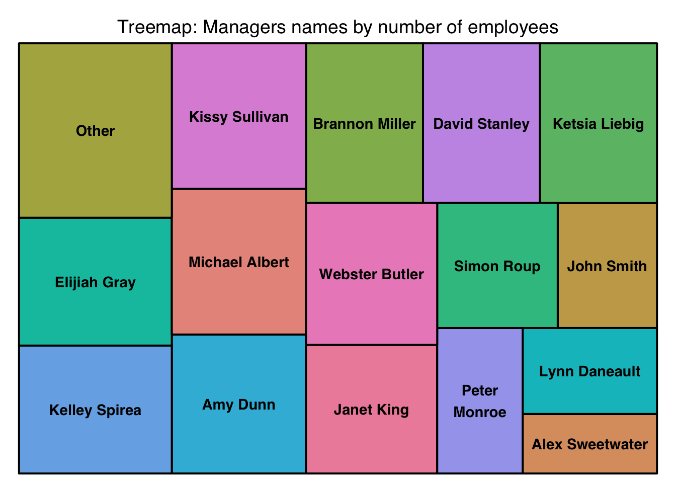
Chicklet chart
term_employees %>% head() %>%
    miss_var_summary()
## # A tibble: 35 × 3
## variable n_miss pct_miss
## <chr> <int> <dbl>
## 1 last_performance_review_date 6 100
## 2 days_late_last30 6 100
## 3 employee_name 0 0
## 4 emp_id 0 0
## 5 married_id 0 0
## 6 marital_status_id 0 0
## 7 gender_id 0 0
## 8 emp_status_id 0 0
## 9 dept_id 0 0
## 10 perf_score_id 0 0
## # … with 25 more rowsterm_employees %<>% select(-last_performance_review_date,
-days_late_last30)
term_employees %>% select(dateof_hire, dateof_termination)## # A tibble: 102 × 2
## dateof_hire dateof_termination
## <chr> <chr>
## 1 9/26/2011 09/25/13
## 2 8/15/2011 08/02/14
## 3 7/7/2014 09/05/15
## 4 3/7/2011 10/31/14
## 5 7/7/2014 09/12/15
## 6 2/16/2015 03/15/15
## 7 2/16/2015 02/22/15
## 8 12/1/2014 05/01/16
## 9 1/5/2015 10/31/15
## 10 1/9/2012 11/04/15
## # … with 92 more rowslibrary(lubridate)
term_employees %<>% mutate(
dateof_hire=anytime::anydate(dateof_hire),
dateof_termination=as.Date(dateof_termination,
format("%m/%d/%y")),
worktime = difftime(dateof_termination, dateof_hire)
)
term_employees %>% select(position, worktime) %>%
mutate(position=as.factor(term_employees$position),
worktime = as.integer(worktime)) %>%
group_by(position) %>% summarise(
avg = round(mean(worktime),0)) %>%
arrange(desc(avg)) %>%
ggplot(aes(x=reorder(position,avg), y=avg)) +
ggchicklet::geom_chicklet(aes(fill=avg),
width = 0.8, radius = grid::unit(5, "pt")) + coord_flip() + scale_fill_gradient(low = '#4B3F72',
high = '#7C9EB2') +
coord_flip() +
scale_y_discrete(expand = c(0, 0)) +
labs(title = "Number of days before quitting job",
subtitle = "By position",
caption = "Data: Kaggle",
fill = "Days") +
theme(
aspect.ratio=4/3,
plot.title = element_text(face = "bold",
size = 13,
family = "Times",
colour = "black"),
plot.subtitle = element_text(size = 11.7,
family = "Times",
colour = "grey45"),
plot.caption = element_text(size = 10,
family = "Times",
colour = "grey45"),
axis.text.y = element_text(vjust = 0.5,
family = "Times"),
axis.title.x = element_blank(),
axis.title.y = element_blank(),
axis.ticks = element_blank(),
axis.line = element_blank(),
panel.grid.major.y = element_blank(),
panel.background = element_blank(),
panel.grid = element_blank(),
panel.border = element_blank(),
legend.justification= c(1,0),
legend.key.size = unit(15, "pt"),
legend.text = element_text(size = 10,
family = "Times"),
legend.position = c(1,0))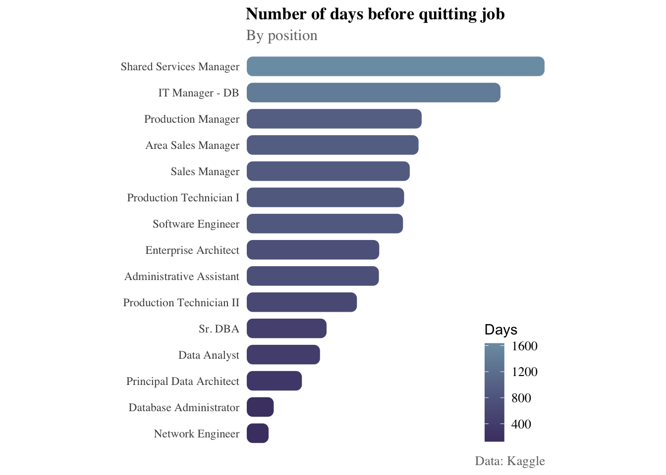
Time series of people quitting
term_employees %>% select(dateof_hire,
    dateof_termination, worktime,
    employee_name,term_reason) %>%
    arrange(worktime) %>% filter(
    worktime < quantile(worktime, 0.05) |
    worktime > quantile(worktime, 0.95)) %>%
    mutate(term_reason = str_to_title(term_reason))
## # A tibble: 12 × 5
## dateof_hire dateof_termination worktime employee_name term_reason
## <date> <date> <drtn> <chr> <chr>
## 1 2012-09-24 2012-09-26 2 days MacLennan, Samuel Hours
## 2 2011-01-10 2011-01-12 2 days Baczenski, Rachael Another Position
## 3 2015-02-16 2015-02-22 6 days Hernandez, Daniff No-Call, No-Show
## 4 2014-02-17 2014-02-25 8 days Evensen, April No-Call, No-Show
## 5 2011-11-07 2011-11-15 8 days Gerke, Melisa Hours
## 6 2011-05-16 2011-06-04 19 days Power, Morissa Another Position
## 7 2011-01-10 2016-01-26 1842 days Robinson, Alain Attendance
## 8 2011-01-10 2016-04-01 1908 days Jung, Judy Unhappy
## 9 2011-01-10 2016-05-17 1954 days Robinson, Cherly Attendance
## 10 2009-10-26 2015-04-08 1990 days Sloan, Constance Maternity Leave …
## 11 2010-10-25 2016-05-18 2032 days Peterson, Ebonee Another Position
## 12 2008-09-02 2015-09-29 2583 days Ybarra, Catherine Another PositionNetwork Visualization
library(igraph)
library(networkD3)
employees %>% select(manager_name, employee_name) %>% head(30) %>% simpleNetwork(
    fontSize = 13, charge = -15,
    linkDistance = 65, zoom = T,
    nodeColour = 'red',
)